Approach

The QuickBot is an inexpensive, differential-drive robotic platform that is easy to build at home, and the MATLAB-based Sim.I.am simulator by Jean-Pierre de la Croix is a simulation environment based around the QuickBot that allows for the rapid development of planning and control algorithms; this makes the QuickBot a great robotic platform for basic controls experimentation. Although the majority of this project is based around the control of a particular robot, much of the work generalizes to any differential drive robot, and even robotics more generally.

Motion Planning

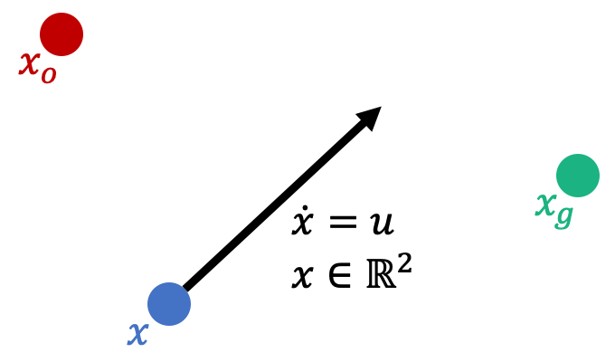
Consider a point on the plane with dynamics governed entirely by a control signal – a “point robot.” This extremely simplified model will be used to develop behaviors (controllers) that, when properly combined, will avoid obstacles and direct the robot to a goal point. This, in effect, will constitute a sort of motion planning system; the hope is that the trajectory generated using this simplified approach can be tracked adequately well given the differential constraints under which the real differential drive robot must operate.

A more sophisticated approach might involve treating the configuration space of the robot as a manifold embedded in a higher-dimensional Euclidean space. The motion planning problem would then become the problem of finding a trajectory that connects the current configuration (a point on the manifold) to the desired configuration (another point on the manifold) that avoids obstacles (global constraints) and restricted velocities (local, differential constraints). This, however, is not the paradigm used for this project; instead, simple controllers are developed in isolation and later stitched together by virtue of a finite state machine to create a complete navigation architecture.

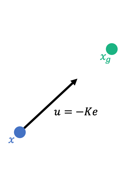
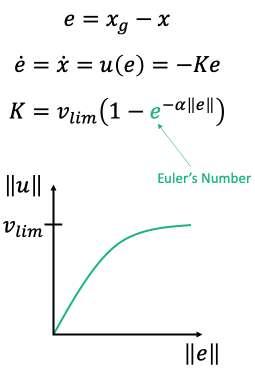
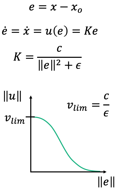
A go-to-goal behavior is developed via vectorial subtraction of the robot position from the goal point, with a gain scaling function that delivers a limited velocity when far from the goal, but reduced velocity when near the goal.

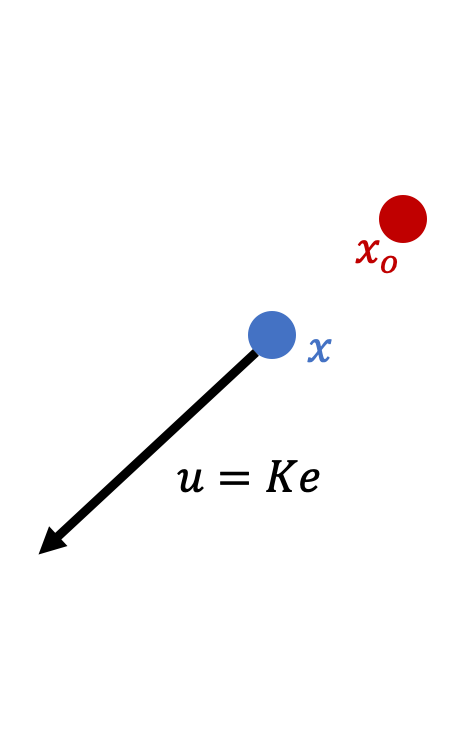
The obstacle avoidance behavior is developed in a manner similar to the go-to-goal behavior: via vectorial subtraction of the obstacle point from the robot position. However, the proposed control law now seeks to destabilize the error dynamics, driving the robot infinitely far away from the obstacle. The gain scaling function is designed to deliver maximum velocity when near the obstacle, and reduce the magnitude when far away from the obstacle.

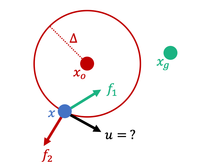
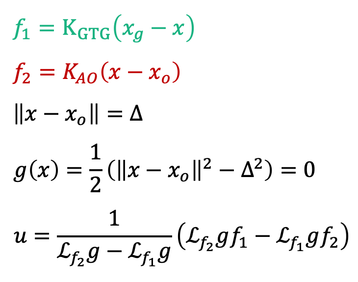
Finally, to negotiate non-convex collections of obstacles, and to address the regime of operation between go-to-goal and obstacle avoidance, a sliding mode controller is developed that balances the opposing vector fields generated by the two other behaviors.

Finite State Machine

When should the robot exhibit a particular behavior over another? An additional architecture is needed to arbitrate the use of specific controls. These modes of operation (the behaviors or control laws) correspond to discrete states that are encoded in what is known as a finite state machine.

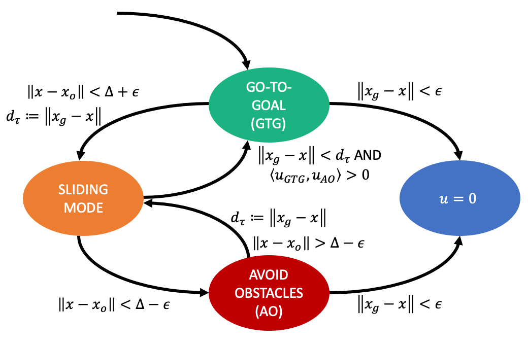
The image above illustrates the QuickBot’s switching logic. The robot starts in the go-to-goal state (green), and terminates when the robot is within an ε-ball of the goal (blue). If the robot’s position is within Δ+ε of an obstacle, it enters the sliding state (orange) and resets the last known displacement from the goal, d_τ, to the current displacement from the goal. If the robot’s position is within Δ-ε of an obstacle, it moves to the avoid obstacles state (red) to avoid imminent collision, and only exits when either the goal is reached or if the robot has achieved a safe distance from the obstacle. Finally, while in the sliding state, if the current distance to the goal is smaller than the last known distance, and the inner product of the go-to-goal and obstacle avoidance vectors indicate that there may be a clear path to the goal, then the robot transitions back to the go-to-goal state.

Robot Model

The point robot presented thus far is obviously not a good model of the QuickBot – it fails to take into account the relationship between the wheels and base motion, as well as robot geometry – and it’s certainly not clear how the control input to the point robot maps to the motor commands that must be delivered to the QuickBot. The goal now is to find this mapping between the point robot and a differential drive robot.

First, an important aside: kinematic models for mobile robots map wheel angular velocities to robot velocities, while dynamic (or sometimes kinetic when more explicit differentiation from kinematic is desired) models map wheel torques to robot accelerations. For the purposes of this project, I only considered kinematic, slip-free models of robot motion.

The unicycle model is a very simple model of a robot that only slightly complicates the point robot model: it adds a heading angle measured with respect to some world frame of reference. The velocity and heading angle are the inputs to the model.

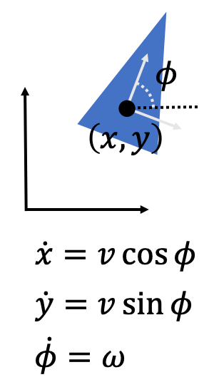
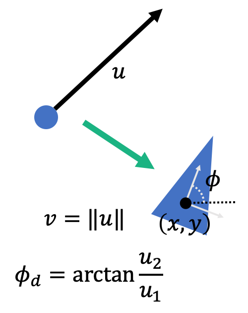
Fortunately, there exists a rather simple mapping between the point robot and the unicycle.

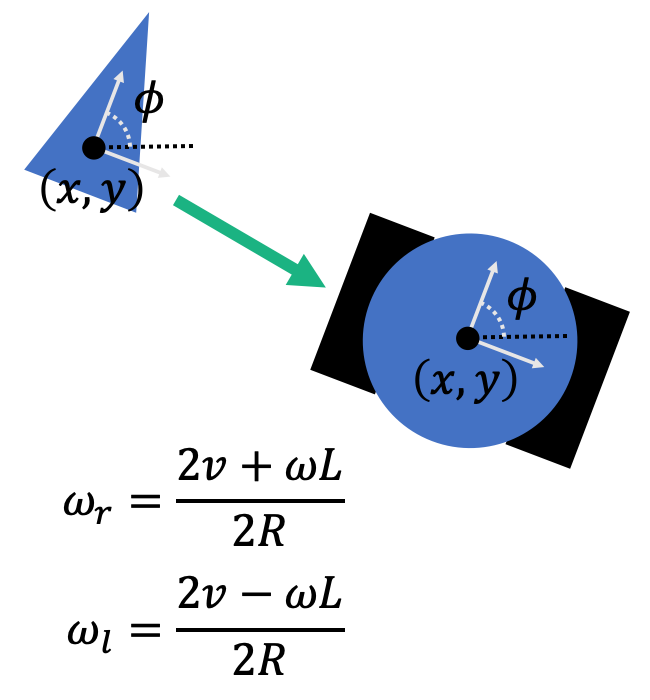
A basic differential drive robot complicates the unicycle model by accounting for the effect that the tire radius, R, and track, or distance between tires, L, has on the position and orientation of the robot. This kinematic model also constitutes a reasonable approximation of how the QuickBot really behaves. Here, the wheel angular velocities are taken to be inputs.

By setting their constitutive differential equations equal to each other, a mapping between the unicycle and the differential drive models is obtained.

For the purposes of this project, it is assumed that the wheel motors are sufficiently powerful and responsive that any wheel angular velocity commanded (below the maximum specified by the motor manufacturer) is attained practically instantly. A consequence of this assumption is that only the robot heading angle must be controlled.

Control

The desired trajectory is determined by the velocity of the point robot; this establishes a desired speed and heading. Since desired speed and actual speed are assumed to be equal, then only the heading angle requires a controller. For this, I use a proportional-integral-derivative (PID) controller.

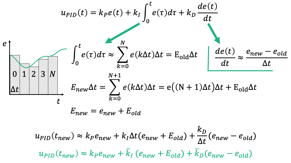
The proportional term in a PID control law scales with the error. The integral term integrates the error over time such that persistent nonzero error increases the magnitude of the integral term, which tends to drive the total error to zero. The derivative term scales with the time rate of change of the error, which provides a sort of forecast of the control required to drive the error to zero. However, when a PID control law is instantiated in a digital computer, care must be taken to convert the proposed PID control law, which is continuous, to the analogous control to be run on the computer, which is discrete.

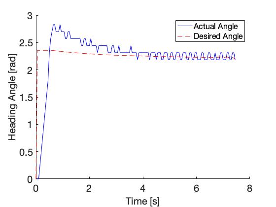
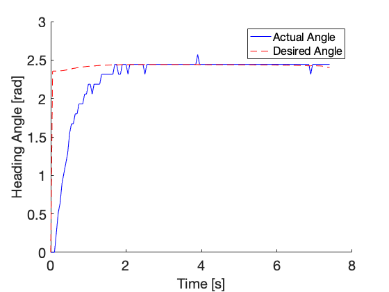
Once the control law is properly implemented on the robot, the PID parameters can be selected (tuned) to achieve good tracking of the heading angle; I do this iteratively via simulation.

Finally, one must account for motor saturation in order for the robot to perform properly. There are situations that could arise in which the desired linear and angular velocities demand a motor output that is beyond the limitations of the motor hardware; in this case, I prioritize steering by reducing the linear velocity until there is enough command headroom to achieve the desired angular velocity. Qualitatively, this means that the robot tends to slow town when making sharp turns, which is a desirable behavior if you don’t want a robot that tips over or regularly slips on the ground.

The Complete System

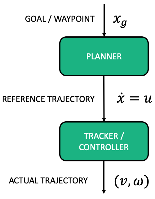
To recapitulate the work thus far: given a goal and a current robot position, the point robot model is used to generate (plan) a trajectory for the QuickBot to follow. Although it might not seem like much of a planner since the entire trajectory is never explicitly computed at once – only the desired speed and heading at an instant in time – the finite state machine does indeed implicitly describe a vector field, and the flow on that field from the starting point to the goal point represents the desired (planned) trajectory. The desired trajectory is given to the tracking system, which transforms the input from the point robot model to the differential drive model and attempts to track those inputs using PID control. The result is the actual trajectory of the QuickBot, which (hopefully) looks very much like the desired trajectory.

When all the mathematics are worked out, and the code is debugged, it’s always nice to see a system behave as intended:

There were many other details that were left out in this (already quite long) project summary – including the properties of the robot sensor skirt, homogeneous transformations between coordinate frames, derivation of the odometry equations, and considerations for continuous (as opposed to point) obstacles – that were nonetheless important in connecting the academic practice of controls to implementation in real systems. Unsurprisingly, it turns out that there are many such steps in manifesting real control systems beyond solving a regulator problem on paper, and they’re a lot of fun (and a lot of work) to carry out.