Approach

A cantilevered beam constitutes the heart of the pumping mechanism where it acts like a large lever. On the tip of the beam is a magnet that, under the forcing caused by a changing magnetic field, oscillates to deform a flexible diaphragm below the center of the beam.

The diaphragm encloses a chamber that contains inlet and outlet ports, each with check valves arranged such that air flows from the inlet to the outlet. The diaphragm and chamber are together modeled as a piston and cylinder arrangement.

The check valves are an inherently nonlinear component; they permit flow in a single direction only, and no flow otherwise. Because of this, extra care must be taken when creating the linear graph or bond graph to ensure the appropriate causality. To better understand why, consider a simple piecewise linear model for the inlet check valve:

In this case, the flow is well-defined: given a pressure drop across the inlet check value, a corresponding flow rate can be computed. However, this function is also not invertible; because of this, the causal chain in the graphs must enforce a specific causality. This implies omitting the check valve dissipating elements from the normal tree (linear graph) and ensuring derivative causality on the dissipating elements (bond graph).

Major Assumptions

Modeling is as much an art as it is a science; mathematical models are, initially, a product of intuition and guesswork since one typically cannot know a priori all of the salient factors that influence the behavior of a model with great certainty until empirical work is carried out. Making a model is, therefore, a sort of back-and-fourth between proposing the underpinnings of a system and corroborating that proposal with experimentation until the model is adequately predictive. Of course, many models have been proposed for many different systems, so starting with secondary research for the system of interest is always helpful when developing a model, as is access to extant empirical data for validating a modeling hypothesis.

To make the guesswork part of model development more explicit, I like to enumerate all of the major modeling assumptions I plan on making before creating a model consistent with those assumptions; if the model fails to predict reality in the way I’d like, I can then turn my attention to the list of assumptions to try to determine which one may not be valid.

Some of the most consequential assumptions for the pump model are:

• Transduction elements are ideal (lossless).
• Capacitance in the electrical domain is taken to be negligible, and inductance is considered only insofar as it contributes to the transducer; this leaves a purely resistive electrical network.
• Magnet travel subtends a small enough angle that its travel can be considered to translate along a line.
• Considering the small travel of the magnet, the constitutive electromagnetic transducer relation is taken to be linear in nature.
• Again, considering the small travel of the magnet, the lever system in which the magnet sits is considered to act in a purely translational manner; that is, rotation is ignored.
• Mechanical components are rigid unless stated otherwise.
• Inertia of the lever is negligible compared to the inertial of the magnet; or, the inertia of all components is accounted for in the magnet inertia.
• Damping effects of the plain rotary bearing are negligible.
• The compliant diaphragm acts as a piston with an effective area not necessarily equal to the area of the circular cross-section of the pumping chamber; this effective area would most easily be found via experimentation, but could also be approximated using a large deformation structural model.
• The compliance of the diaphragm can be modeled as a linear spring.
• The damping caused by the deformation of the diaphragm almost certainly contributes to a significant amount of energy loss for the system; however, all losses will be considered in the fluid domain only.
• The fluid resistance of the check valves will be considered alone. All fluid resistances outside of the check valves (e.g. the filter) can either be considered negligible, or can be considered to contribute to the effective resistances of the check valves.
• Fluid resistance is assumed to behave linearly (porous plug flow).
• Fluid compressibility effects in the chamber are significant, and can be modelled as linear fluid capacitance.
• Fluid inertance is ignored.

Variable Definitions

E_IN – The input voltage, applied to the coil

R_C – Coil winding resistance

i – Current in the coil

K – This coefficient relates the electrical domain to the mechanical domain. It is often approximated using the product of the magnetic field strength, the “effective length” of the coil, and the number of wire turns in the winding.

m – magnet mass

V_m – velocity of the magnet mass

F_m – force on magnet mass

A (as a subscript) – a point on the lever mechanism defined as the location of attachment of the diaphragm

B (as a subscript) – a point defined as the magnet end of the lever mechanism, also assumed to be the same point as the effective center of mass of the magnet

V_p – velocity of the piston

k_p – linear spring stiffness of diaphragm

A – effective area of the piston. Because the diaphragm deforms in order to displace fluid, this is not necessarily equal to the inner diameter of the chamber. It is, perhaps, best to measure this relationship between displacement and volumetric flow rate (or force and pressure) empirically. Can be estimated by assuming by assuming a geometry of deformation.

C – fluid (air) compliance. Can be determined using an ideal gas law. In our case, it can be estimated by C=V⁄nP, where V is the volume of the chamber, n is the polytropic index, and P is the pressure.

R₁ – linear fluid resistance of the input check valve. This may also be considered to be the sum of all resistances on the input side.

R₂ – linear fluid resistance of the output check valve. This may also be considered to be the sum of all resistances on the output side.

p_c – chamber pressure

P_IN, P_OUT – input and output pressure, respectively

e₁, F₁, F₂, Q₃ – “placeholder” variables, used to complete transducer constitutive relationships

Note that the above list of variables is not necessarily exhaustive; however, the meaning of any variable introduced later should be clear in context.

Linear Graph

The term linear graph refers to a graphical representation of a system and also a generic, multi-domain, graphical modeling technique that could be considered a generalization of electrical circuit models – in fact, when you look at a linear graph, you’re very nearly looking at an equivalent circuit model. Rules for finding the normal tree are used to determine independent energy storage elements, which constitute the system states. Equations that arise from application of the compatibility condition (a generalization of Kirchhoff’s voltage law) and continuity condition (a generalization of Kirchhoff’s current law) allow for algebraically finding the state equations. Care is taken to avoid causality conflicts and algebraic loops, which often arise from poor modeling assumptions and are not always immediately obvious when modeling multi-domain systems.

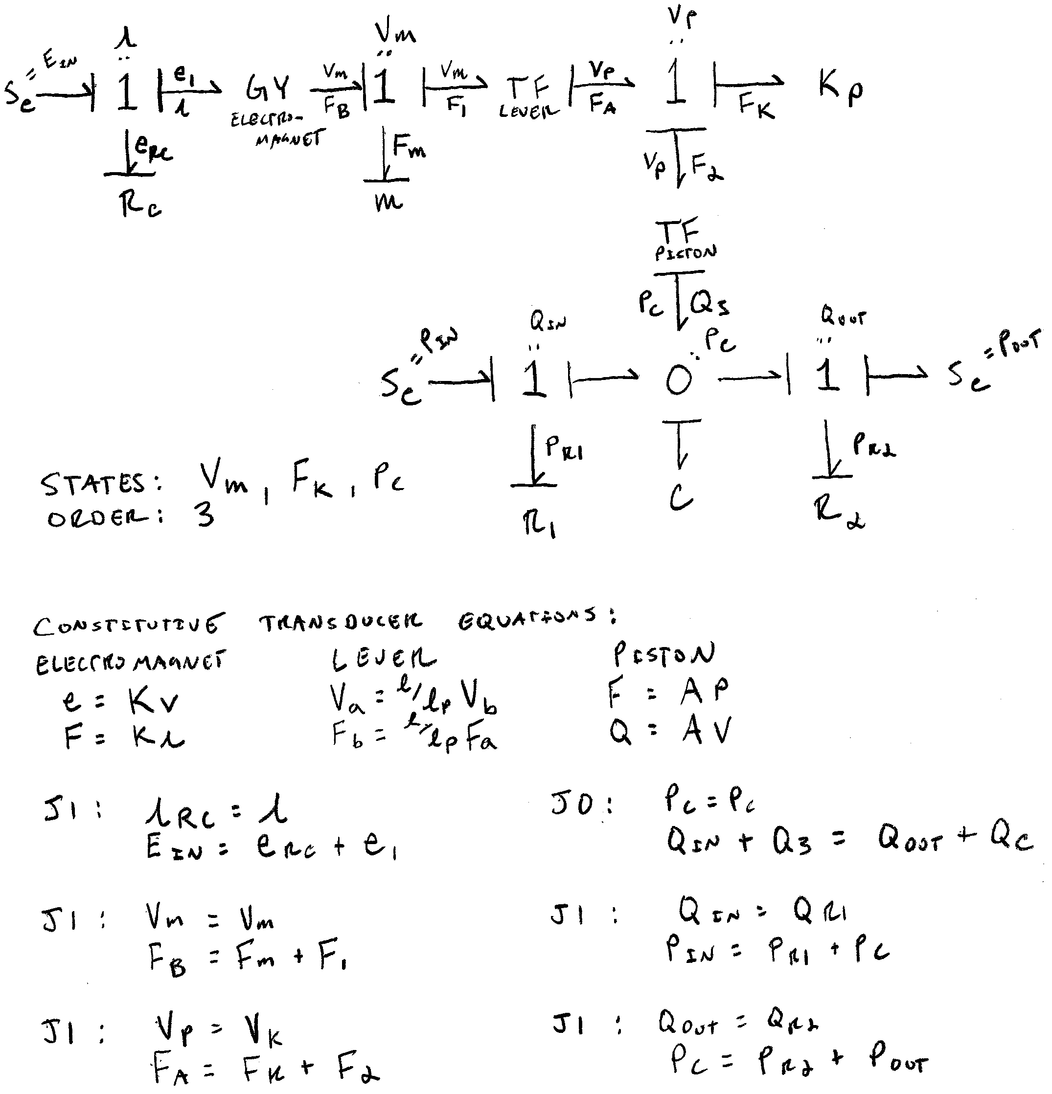
Bond Graph

As with a linear graph, the term bond graph refers to both a graphical representation of a dynamical system as well as a generic, multi-domain, graphical modeling technique that aids in the understanding of systems and in the derivation of the state equations. Elements in the graph are connected with bonds that represent bi-directional exchange of energy. Similar to identification of the normal tree with linear graphs, causality assignment is used to determine the independent energy storage elements in the system and thus the state variables. Compatibility and continuity conditions allow for the algebraic isolation of the state variables. Care is taken to avoid causality conflicts and algebraic loops, which often arise from poor modeling assumptions and are not always immediately obvious when modeling multi-domain systems.

State Equations

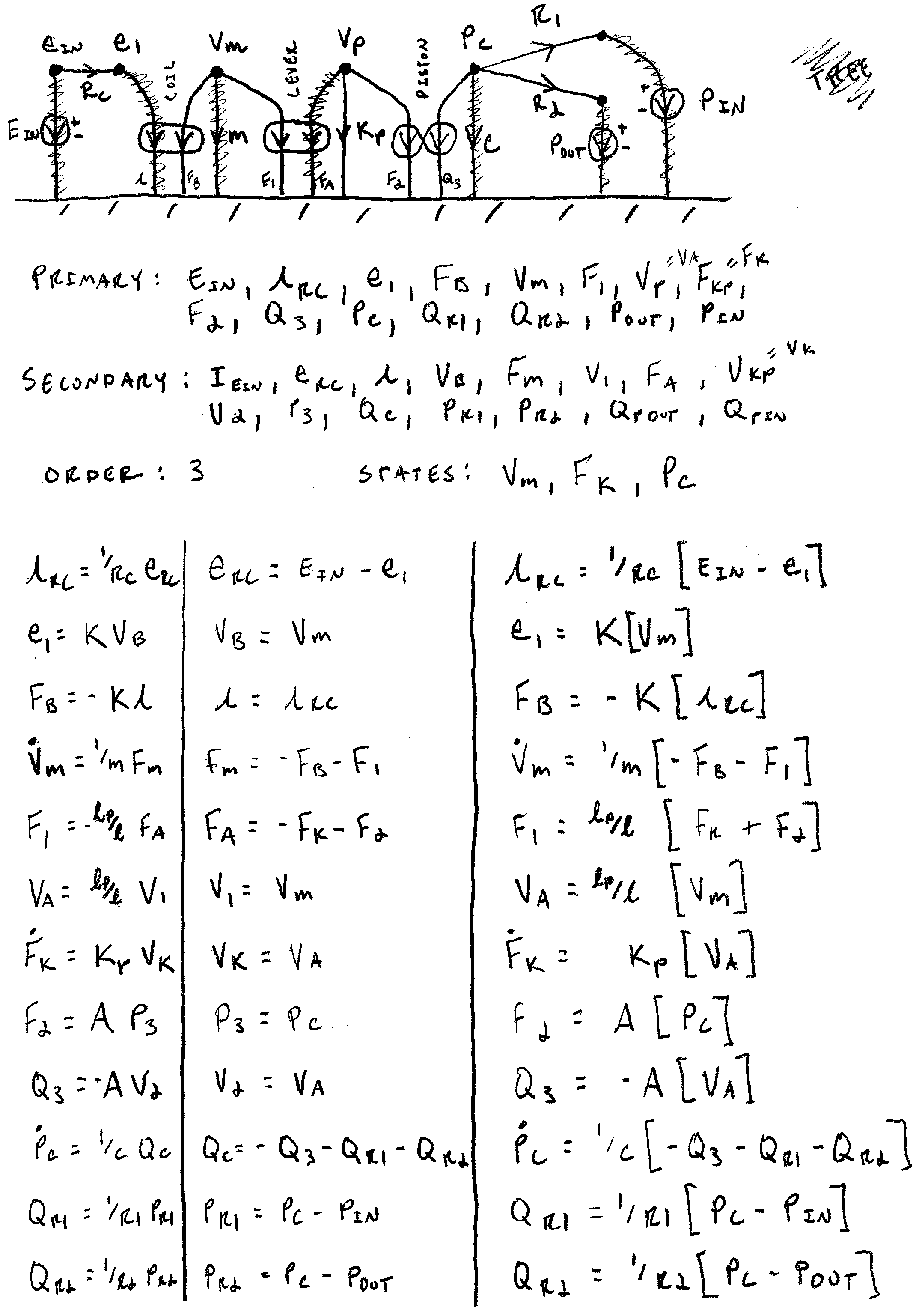
Either the linear graph or bond graph may be used, together with the element and transducer constitutive relations, to derive a state-space representation of the system. Most of the nonlinearities in this system were neglected for the sake of keeping a toy problem simple; assume for a moment we may treat the check valves in the same manner. Then, the state-space representation may take the familiar matrix form:

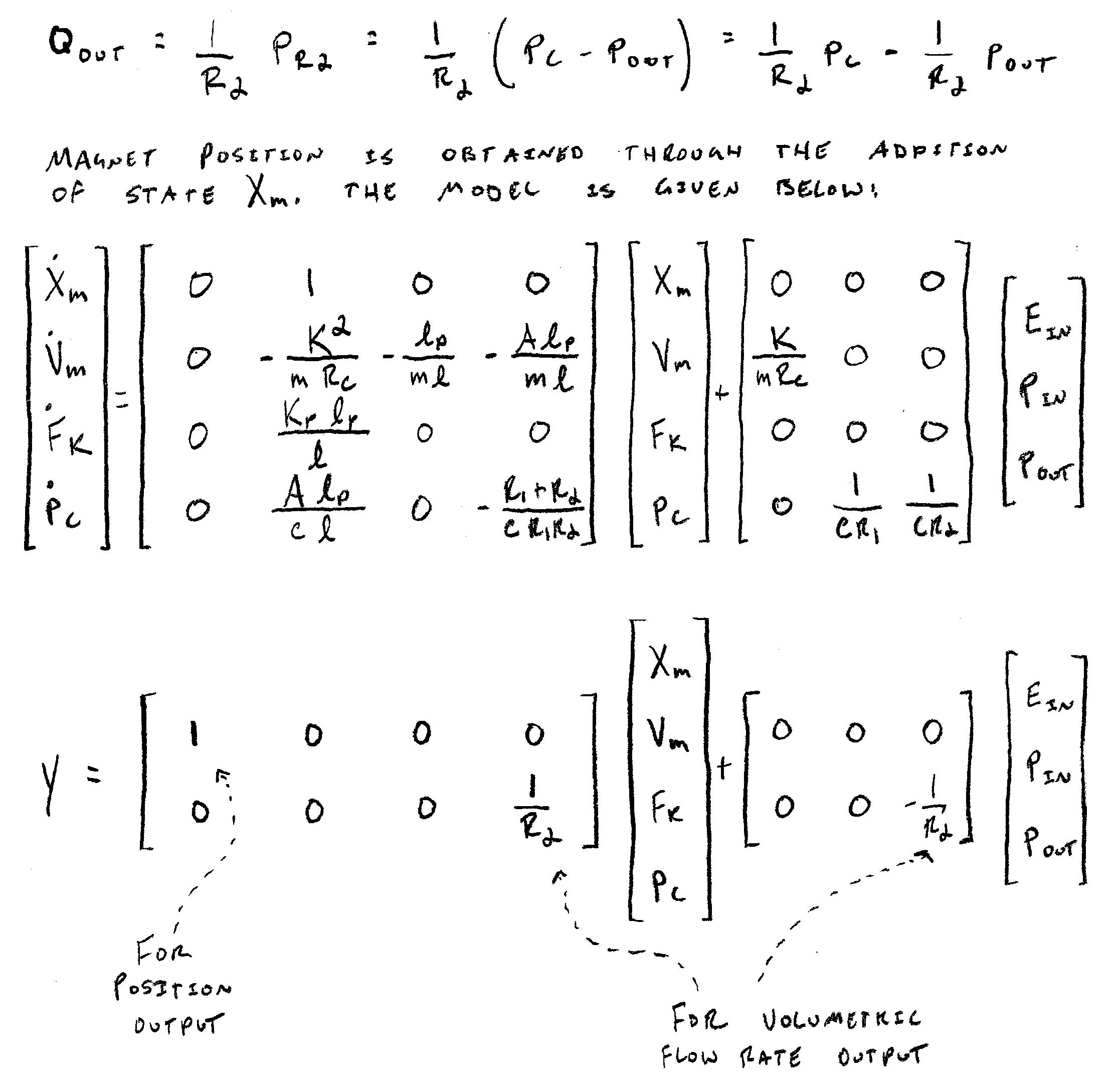
In this case, a state was added to track the displacement of the magnet in the output. Also, an additional output equation was derived to track the output volumetric flow rate of the pump, which seems useful as a design variable for a pump model.

Of course, for a real model to be useful, the piecewise linear check valve model would need to be incorporated, which also means that the system cannot be written in matrix form. In this case, it may be more appropriate to choose the volume of the air chamber as a state variable instead of the pressure; this volume could be expressed in terms of the volumetric flow rate variables for the check valves, which can then be computed using the piecewise linear model.