Approach

A building’s structural elements are more closely described by continuous media; why, then, choose a lumped-element model? There are a few reasons:

1. A lumped-element model, represented by Ordinary Differential Equations (ODEs) is simpler to derive and more tractable than a model that assumes continuously distributed elements, which are represented by Partial Differential Equations (PDEs).
2. There is a substantial literature around the solutions to and analysis of systems of ODEs, as well as the control of such systems.
3. Perhaps most importantly, it’s a surprisingly good model of building vibration behavior and has been used even in fairly recent and well-cited research publications!

That being said, I don’t claim to have any specific expertise in structural engineering beyond that which finds home in a mechanical engineer’s education. Caveat emptor!

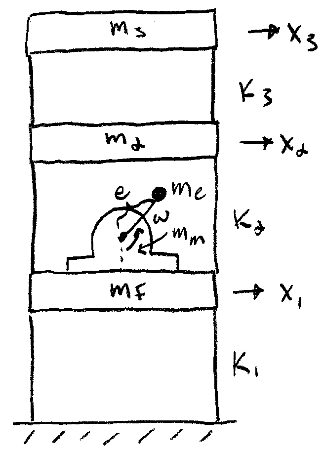
To keep things very simple, consider a building with three floors above ground level, connected by compliant components (the walls and other structures that support the floors) and an unbalanced machine that will provide the vibration input:

Major Assumptions

Modeling is as much an art as it is a science; mathematical models are, initially, a product of intuition and guesswork since one typically cannot know a priori all of the salient factors that influence the behavior of a model with great certainty until empirical work is carried out. Making a model is, therefore, a sort of back-and-fourth between proposing the underpinnings of a system and corroborating that proposal with experimentation until the model is adequately predictive. Of course, many models have been proposed for many different systems, so starting with secondary research for the system of interest is always helpful when developing a model, as is access to extant empirical data for validating a modeling hypothesis. In this case, ample work exists in the lumped-element modeling of buildings that may be drawn upon for model parameter population and validation.

To make the guesswork part of model development more explicit, I like to enumerate all of the major modeling assumptions that I plan on making before creating a model consistent with those assumptions; if the model fails to predict reality in the way I’d like, I can then turn my attention to the list of assumptions to try to determine which one may not be valid.

Here are some of the more consequential assumptions I make for the building model:

• Massless springs (i.e., walls and floor supports are massless, or assume that equivalent additional wall mass is added to each floor mass)
• Deflections are small such that only horizontal motion of the floors need be considered.
• Angular velocity of the motor is an independent input; that is, there is no backwards coupling from the floor motion to the motor.
• Linear elastic behavior in the range of motion considered in the model
• Forces in the vertical direction are ignored.
• The floors act as point masses (this is essentially a restatement of some of the assumptions above; in this way, we need not consider general planar rigid body motion).

Variable Definitions

m_f – mass of second floor (the driven floor)

m_m – mass of the machine (less the eccentric mass)

m_e – mass of eccentric mass

e – radial distance from rotating center to eccentric mass

ω – angular velocity of motor output

k₁, k₂, k₃ – stiffness of each set of wall and floor supports

x₁, x₂, x₃ – absolute displacement of each floor (measured from ground frame of reference)

t – time

Also: m₁ = m_f + m_m

Note that the above list of variables is not necessarily exhaustive; however, the meaning of any variable introduced later should be clear in context.

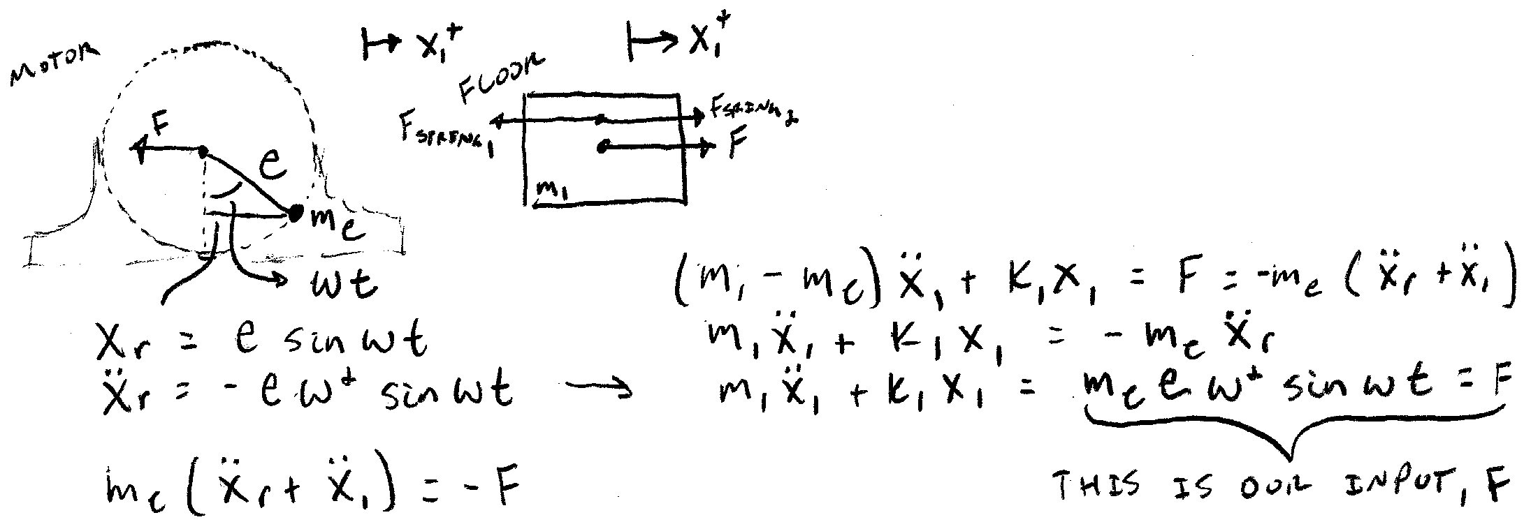
Dynamics of Motor Input

Since backwards coupling from the floor to the unbalanced mass is assumed to be negligibly small, an analysis of unbalanced rotation is carried out to determine the forcing from the motor to the floor.

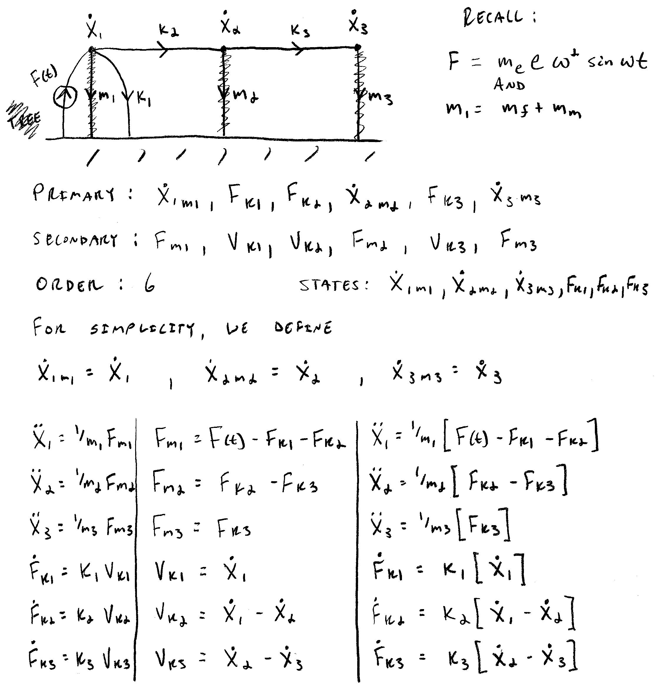
Linear Graph

The term linear graph refers to a graphical representation of a system and also a generic, multi-domain, graphical modeling technique that could be considered a generalization of electrical circuit models – in fact, when you look at a linear graph, you’re very nearly looking at an equivalent circuit model. Rules for finding the normal tree are used to determine independent energy storage elements, which constitute the system states. Equations that arise from application of the compatibility condition (a generalization of Kirchhoff’s voltage law) and continuity condition (a generalization of Kirchhoff’s current law) allow for algebraically finding the state equations. Care is taken to avoid causality conflicts and algebraic loops, which often arise from poor modeling assumptions and are not always immediately obvious when modeling multi-domain systems.

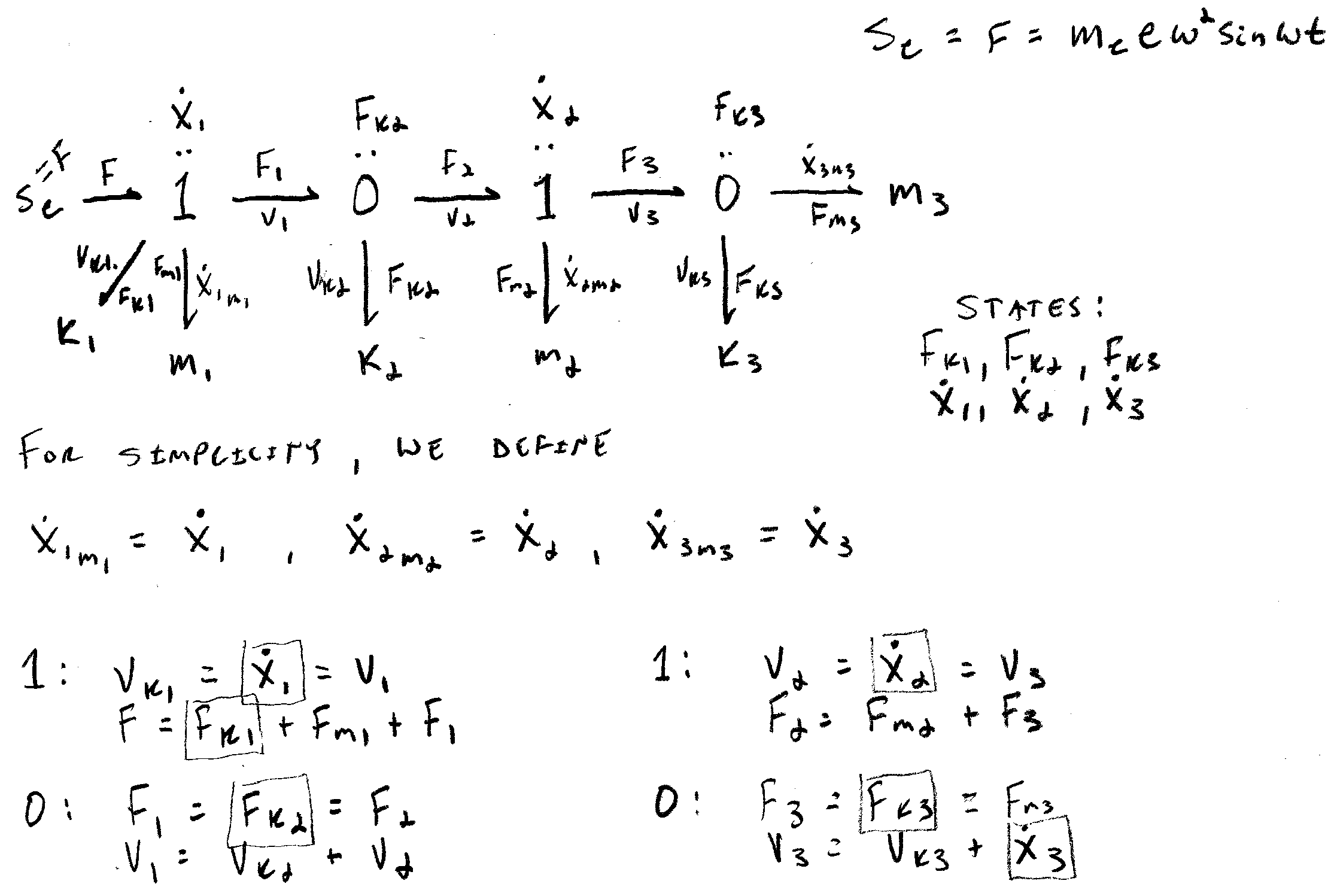
Bond Graph

As with a linear graph, the term bond graph refers to both a graphical representation of a dynamical system as well as a generic, multi-domain, graphical modeling technique that aids in the understanding of systems and in the derivation of the state equations. Elements in the graph are connected with bonds that represent bi-directional exchange of energy. Similar to identification of the normal tree with linear graphs, causality assignment is used to determine the independent energy storage elements in the system and thus the state variables. Compatibility and continuity conditions allow for the algebraic isolation of the state variables. Care is taken to avoid causality conflicts and algebraic loops, which often arise from poor modeling assumptions and are not always immediately obvious when modeling multi-domain systems.

State Equations

Either the linear graph or bond graph may be used, together with the element and transducer constitutive relations, to derive a state-space representation of the system. Since the nonlinearities in this system were ignored for the sake of keeping a toy problem simple, the state-space representation may take the familiar matrix form:

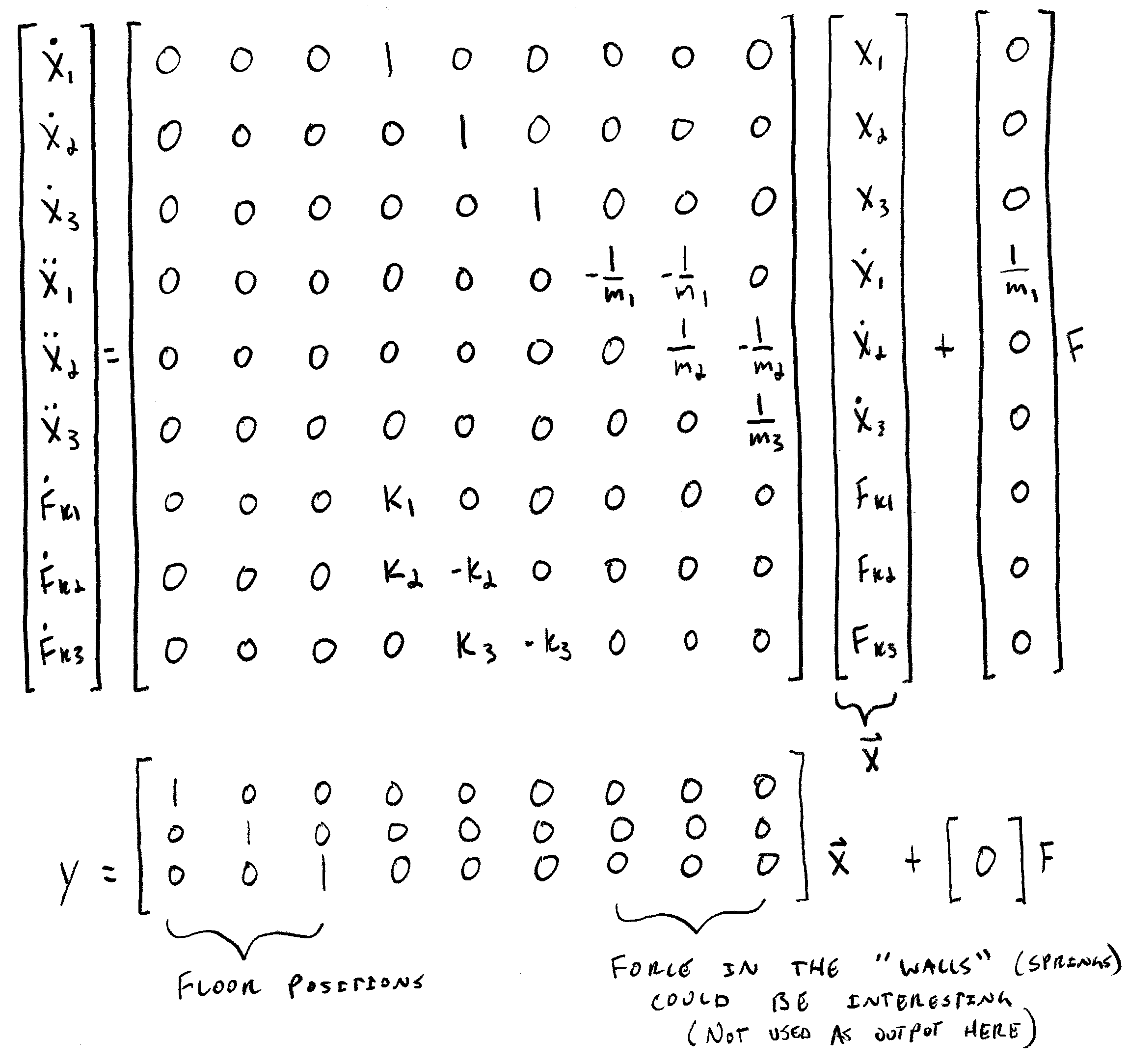
Notice that the system matrix is fairly sparse; the entries appear in a predictable pattern, and the model can be easily extended to an arbitrary number of floors without the need to rederive the state equations from scratch!