Mathematical Model of a VCR
Summary
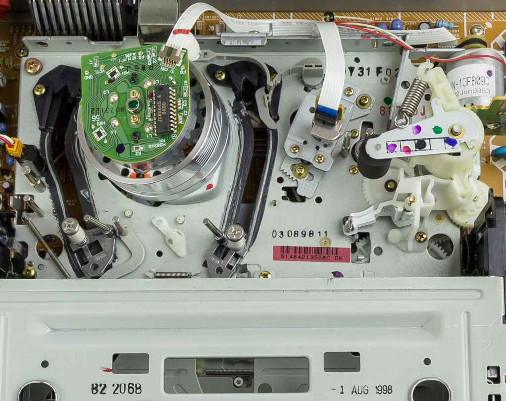
The number of people who have ever heard of a videocassette recorder (VCR) is almost certainly dwindling precipitously, so it might be worthwhile to first explain what a VCR is: a device that sends magnetic tape stored in a cassette through a maze of rollers, passing it over transducers to read and write data. Typically, people used VCRs to record and play back television programming at home. These devices, though obsolete, contain several clever electromechanical solutions to tape management that are satisfying to understand.
Goal
In this informal modeling project, I create a lumped-element mathematical model for part of the chain of components responsible for the magnetic tape routing in a VCR.
Approach
VCRs may seem rather antiquated, but they are anything but simple; during the height of their popularity, VCRs were arguably the most complex domestic electromechanical system – second only, perhaps, to the car. The fact that a VCR could be had for a fraction of weekly pay and could operate for years without maintenance is a testament to the quality of engineering and design work that went into creating these devices.
A mathematical model that tracked every variable of interest in a VCR would be outrageously complex and probably not very useful; instead, I opted to focus on some of the interesting components that drive the tape through the system.
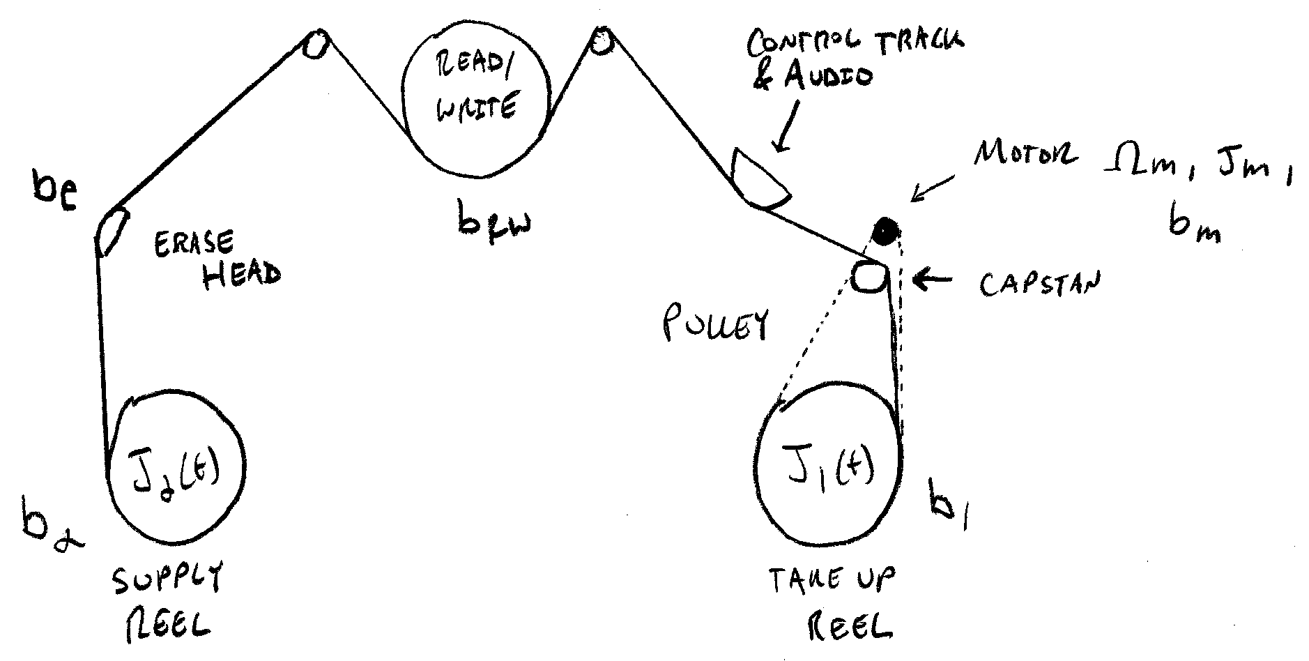
Tape is fed from a supply reel through a series of rollers to make contact with various heads (transducers) that either read or write data to the tape. A capstan and a pinch roller grip the tape just before the supply reel to force the tape to move at a constant speed. Finally, the tape is spooled on the take-up reel.
Here’s a schematic indicating some of the components of interest:
The capstan portion of the system is what drives the tape motion:
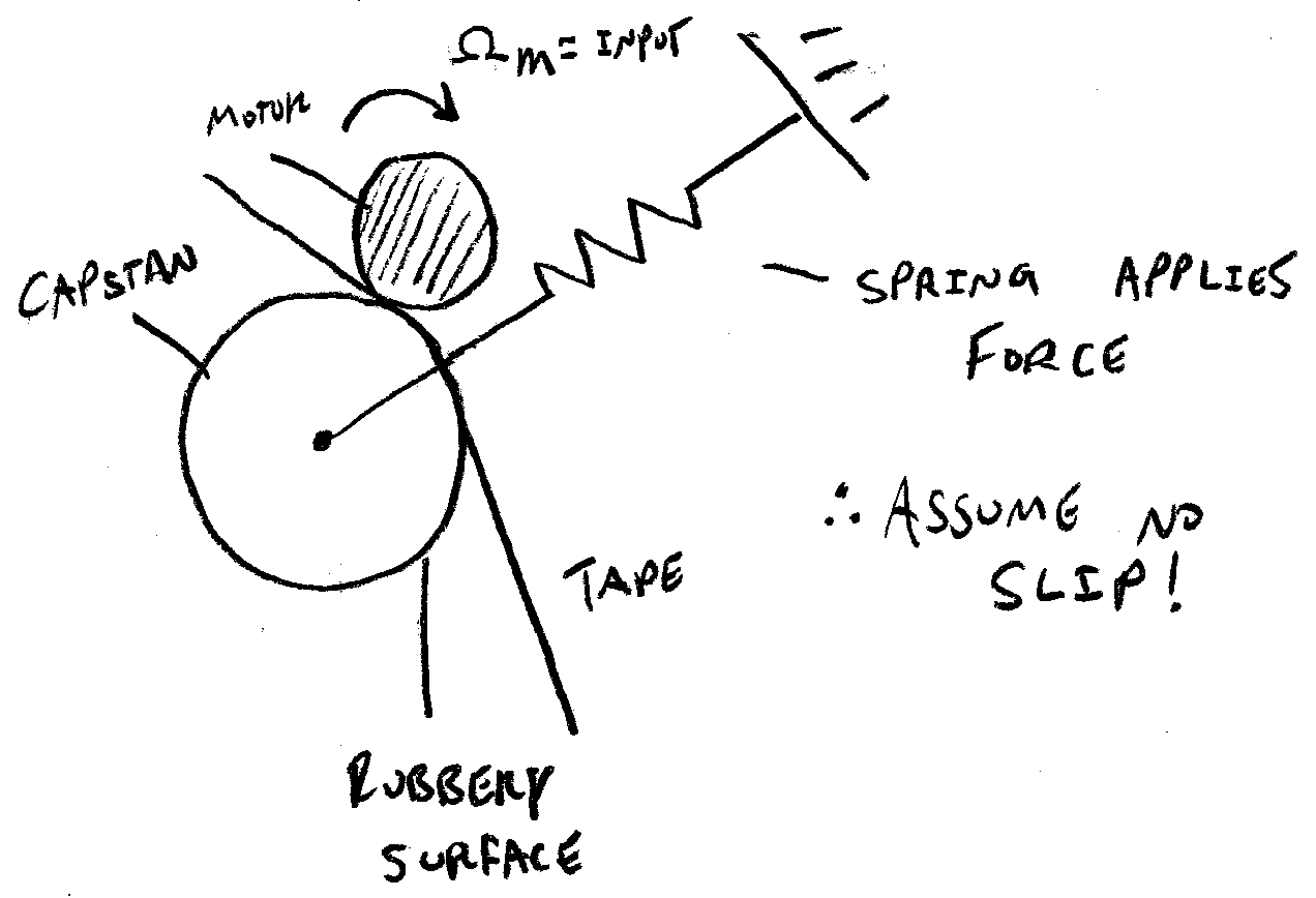
If you’ve been paying attention so far, you might wonder why the capstan system is used at all; why doesn’t one just drive the take-up reel directly with a motor to pull the tape along? The issue with this approach is that the radius of the take-up reel continuously varies as tape spools on the reel; as it gets larger and larger, the linear velocity of the tape would get faster and faster if the reel is driven at a constant rate of rotational. Correcting for this change in radius via motor control would require either precision sensing of the radius of the take-up reel (tricky and expensive) or additional information stored on the tape (reduces useful data storage density). Instead, the capstan – with its fixed radius and high-friction surface – can be driven at a constant angular velocity, pulling the tape along at a constant linear velocity.
However, this doesn’t totally solve the problem; regardless of the mechanism by which the tape is driven, the take-up reel must rotate to spool the tape, and the rate of rotation must change as the take-up reel radius changes. To address this, engineers used a very elegant, low-tech solution involving a belt drive.
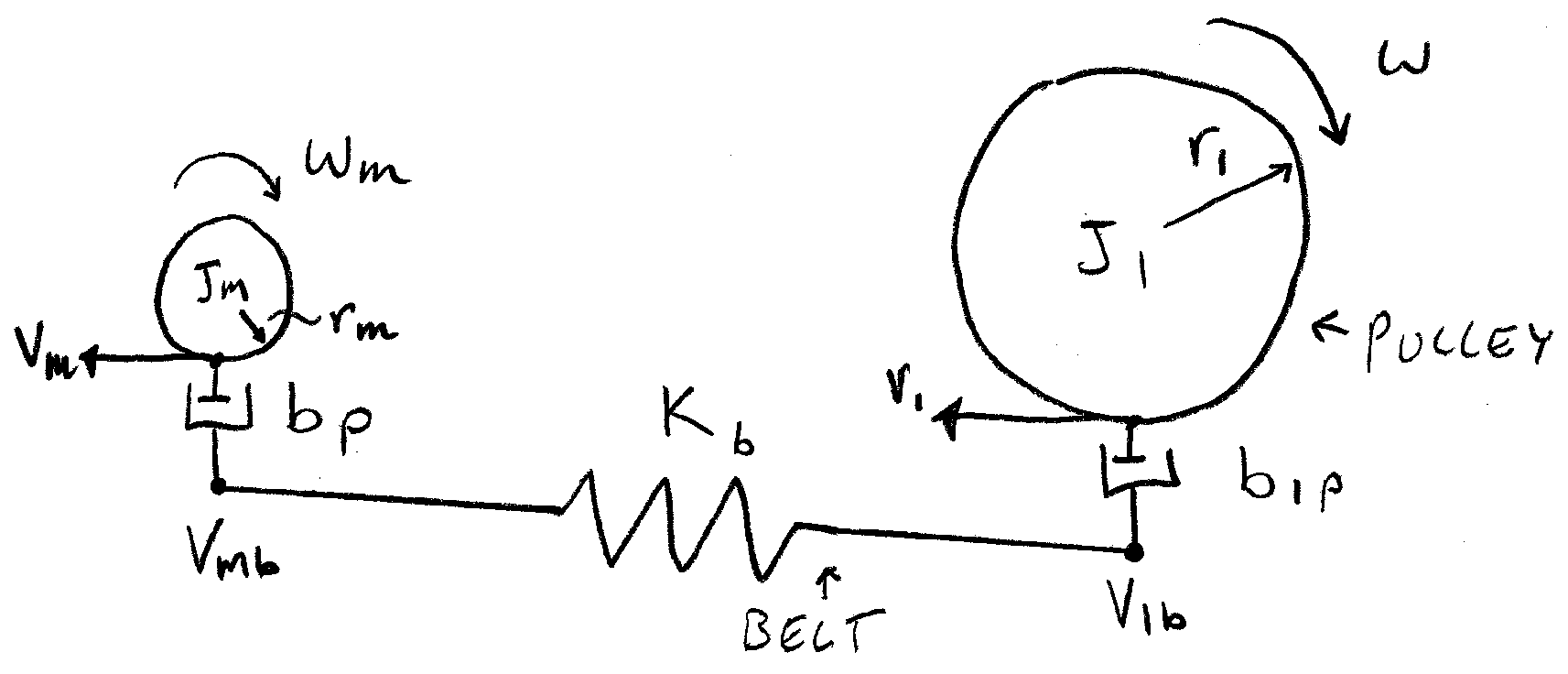
The idea is to connect the capstan motor to the take-up reel by virtue of a belt drive. However, the take-up reel pulley is made of a very smooth material such that the belt easily slips over the take-up reel pully when minimal resistance is encountered. The pulley ratios are selected such that, if the belt operates without slipping, the take-up reel achieves an angular velocity that is higher than would ever be demanded by the capstan. During operation, the magnetic tape provides a torque on the take-up reel pulley that prevents the take-up reel from rotating more than is required; the belt then slips on the pulley, and the rate at which the capstan outputs tape matches the rate at which the take-up pulley spools the tape. Since reel-to-reel systems existed long before the VCR was invented, the VCR does not represent the first instance of such a solution; however, it is a beautiful application of the working principle and I find it quite remarkable how robust the solution is in practice.
The slipping pulleys are modeled using rotational-to-linear transducers, linear viscous damper elements, and a belt compliance. To keep the linear and bond graphs simple below, I decided to relate the tape velocity to the take-up reel only – omitting the torqueing effect of the tape on the reel due to the capstan; however, the model could easily be augmented to capture this effect, if desired.
Major Assumptions
Modeling is as much an art as it is a science; mathematical models are, initially, a product of intuition and guesswork since one typically cannot know a priori all of the salient factors that influence the behavior of a model with great certainty until empirical work is carried out. Making a model is, therefore, a sort of back-and-fourth between proposing the underpinnings of a system and corroborating that proposal with experimentation until the model is adequately predictive. Of course, many models have been proposed for many different systems, so starting with secondary research for the system of interest is always helpful when developing a model, as is access to extant empirical data for validating a modeling hypothesis.
To make the guesswork part of model development more explicit, I like to enumerate all of the major modeling assumptions that I plan on making before creating a model consistent with those assumptions; if the model fails to predict reality in the way I’d like, I can then turn my attention to the list of assumptions to try to determine which one may not be valid.
I make many, rather liberal assumptions about the VCR model; some of the most consequential are:
- Only electrical resistance will be considered in the electrical domain (i.e. no considerable motor capacitance or inductance).
- All components are rigid unless stated otherwise.
- The change in inertia of the take up and supply reels during operation is negligible when compared to the total inertia; in other words, the inertia of the reels is constant.
- The radii of the reels do not change with time.
- All effects of friction may be modelled as linear viscous in nature.
- The equivalent friction from all of the rotating components (besides the motor friction) can be assumed to act at a single linear velocity.
- The tape compliance is negligible between the capstan and the take up reel, but compliance is not negligible between the capstan and the supply reel (the longest run of tape).
- The output motor shaft radius and its pulley radius are the same.
- The tape does not slip through the motor and capstan pinch point.
Variable Definitions
E(t) – input voltage applied to the motor
R – motor winding resistance
iR – current in motor resistance
bm – motor viscous damping coefficient
K – back-EMF (or, equivalently, the torque constant) of the motor
ωJm – motor angular velocity
N1 – radius of the take up reel
N2 – radius of pulley connected to the take up reel
N3 – radius of supply reel
vm – linear velocity of point on the surface of the motor output
vp – linear velocity of the belt attached to the output motor shaft
v1p – linear velocity of the belt attached to the take up reel pulley
J1 – moment of inertia of the take up reel
J1 – moment of inertia of the supply reel
ω1 – angular velocity of the take up reel
ω2 – angular velocity of the supply reel
e1, ea, v1, etc. – “placeholder” variables (used to complete transducer constitutive relationships)
Note that the above list of variables is not necessarily exhaustive; however, the meaning of any variable introduced later should be clear in context.
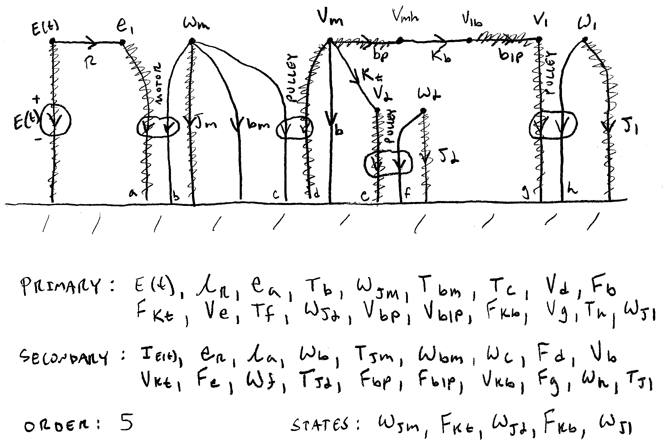
Linear Graph
The term linear graph refers to a graphical representation of a system and also a generic, multi-domain, graphical modeling technique that could be considered a generalization of electrical circuit models – in fact, when you look at a linear graph, you’re very nearly looking at an equivalent circuit model. Rules for finding the normal tree are used to determine independent energy storage elements, which constitute the system states. Equations that arise from application of the compatibility condition (a generalization of Kirchhoff’s voltage law) and continuity condition (a generalization of Kirchhoff’s current law) allow for algebraically finding the state equations. Care is taken to avoid causality conflicts and algebraic loops, which often arise from poor modeling assumptions and are not always immediately obvious when modeling multi-domain systems.
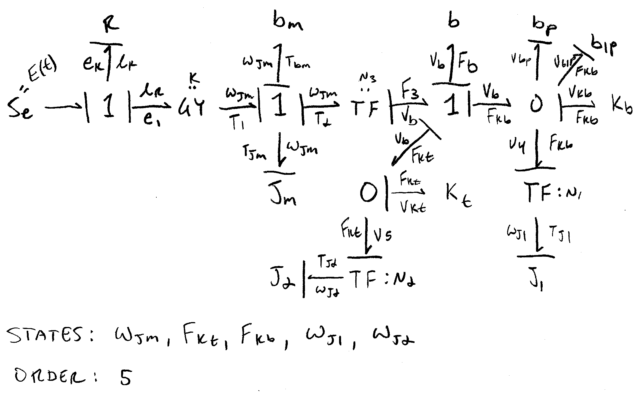
Bond Graph
As with a linear graph, the term bond graph refers to both a graphical representation of a dynamical system as well as a generic, multi-domain, graphical modeling technique that aids in the understanding of systems and in the derivation of the state equations. Elements in the graph are connected with bonds that represent bi-directional exchange of energy. Similar to identification of the normal tree with linear graphs, causality assignment is used to determine the independent energy storage elements in the system and thus the state variables. Compatibility and continuity conditions allow for the algebraic isolation of the state variables. Care is taken to avoid causality conflicts and algebraic loops, which often arise from poor modeling assumptions and are not always immediately obvious when modeling multi-domain systems.
State Equations
Either the linear graph or bond graph may be used, together with the element and transducer constitutive relations, to derive a state-space representation of the system. Since the nonlinearities and time-varying parameters in this system were ignored for the sake of keeping a toy problem simple, the state-space representation may take the familiar matrix form:
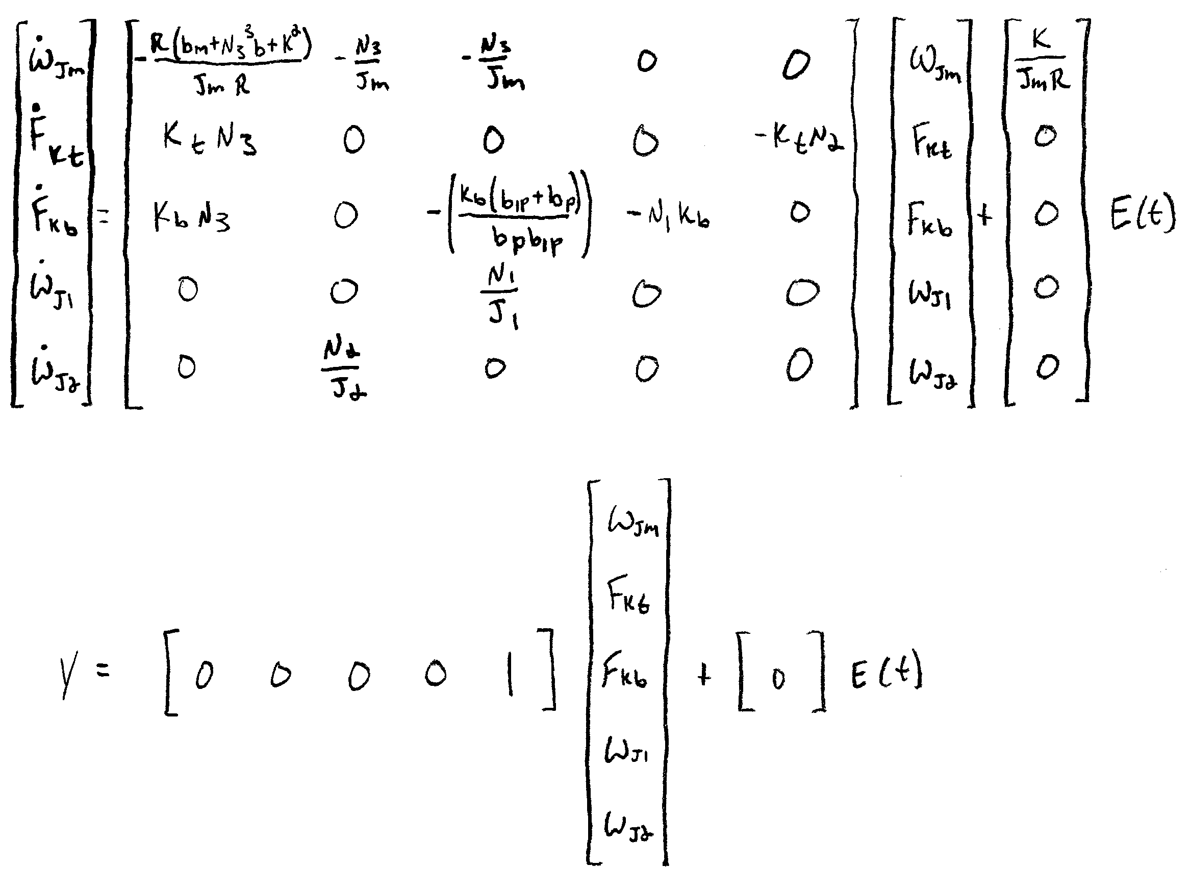
In this case, I decided, arbitrarily, to set the system output to the rotation rate of the supply reel.